목차
데이터

1. 라이브러리
import pandas as pd
import matplotlib.pyplot as plt
import seaborn as sns
import statsmodels.api as sm
from statsmodels.formula.api import ols
2. Data exploration
1) pairplot
---> Radio가 Sales와 가장 강한 양의 상관관계가 있고, Social Media 역시 약하지만 양의 상관관계가 있다. 다만 social media는 radio와 선형관계가 있기 때문에, 설명력이 더 좋은 Radio를 선택하고 social media는 선택하지 않는다.
2) Categorical variables
---> TV의 경우 광고를 많이 할 수록 판매에 강한 영향을 미치며, influencer 같은 경우에는 큰 차이가 없다.
3. Model Building
ols_formula = 'Sales ~ C(TV) + Radio'
OLS=ols(formula=ols_formula, data= data)
model= OLS.fit()
result=model.summary()
4. Model assumption
1) Linearity
fig, axes=plt.subplots(1,3, figsize=(12,4))
sns.scatterplot(x=data['Radio'], y=data['Sales'], ax=axes[0])
sns.scatterplot(x=data['Social_Media'], y=data['Sales'], ax=axes[1])
sns.scatterplot(x=data['Social_Media'], y=data['Radio'], ax=axes[2])

axes[0].set_title("Radio and Sales")
axes[1].set_title("Social Media and Sales")
axes[2].set_title("Social Media and Radio")

plt.tight_layout()
2) Normality
# 잔차
residual= model.resid
residual

# 두 개 그래프 놓을 공간 만들기
fig, axes=plt.subplots(1,2, figsize=(8,4))

# 간격 맞추기
plt.tight_layout()

plt.show()
첫 번째, 히스토그램
# 첫 번째 히스토그램
sns.histplot(residual, ax=axes[0])
axes[0].set_xlabel('Residual Value')
axes[0].set_title("Histogram of Residual")
두 번째, qqplot
#두 번째 qqplot
sm.qqplot(residual, line='s', ax=axes[1])
axes[1].set_title("Normal qqplot")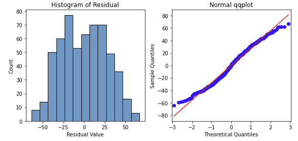
---> 잔차가 정규분포를 이루며, qq plot 역시 곧은 직선 모양이므로 정상성 조건에 만족한다.
3) Independence observations
관찰된 데이터셋에서 각각의 독립변수들이 독립적이다.
4) Constant Variance 등분산성
★ fitted value 예측값
fitted value 의미는 적합값으로 회귀식에 의해 예측된 Y값이다. 즉 예측값이라고 할 수 있다.
fitted value= predicted value
★ residual 잔차
관측값(실제값)과 예측값의 차이
fig=sns.scatterplot(x=model.fittedvalues, y=model.resid)
fig.axhline(0)

fig.set_xlabel("Fitted values")
fig.set_ylabel("Residuals")
fig.set_title("Fitted Values v. Residuals")
plt.show()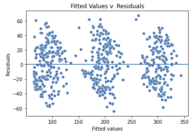
-----> 이 모델에서 TV가 sales값을 결정하는 가장 지배적인 카테고리컬 변수이기 때문에 fitted values 값이 세 가지로 나뉜다. 어찌되었건 세 개의 집단 모두 분산이 동일하게 분포되어 있으므로 이 가정 역시 만족한다.
5) multicollinearity 다중공선성
다중공선성을 진단하기 위해 VIF 지수를 확인할 것이다. 우선 파이썬 VIF 라이브러리 호출한다.
from statsmodels.stats.outliers_influence import variance_inflation_factor
다중공선성이 의심되었던 radio와 social media에 관한 vif 점수를 진단해보자.
X = data[['Radio','Social_Media']]
vif = [variance_inflation_factor(X.values, i) for i in range(X.shape[1])]
df_vif = pd.DataFrame(vif, index=X.columns, columns = ['VIF'])
df_vif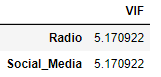
5. 결과 분석 및 해석
1) R 스퀘어(결정계수)
0.904=90.4%
이 모델은 SALES 안의 변동을 90.4% 정도 설명한다는 뜻이고, 이 정도 결과는 매우 훌륭하다.
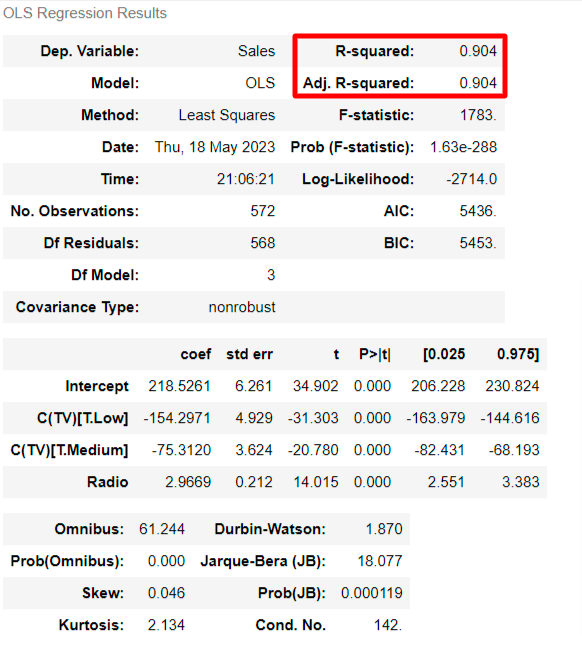
2) 회귀계수
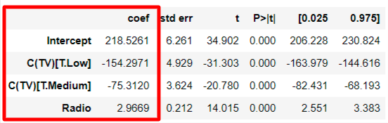
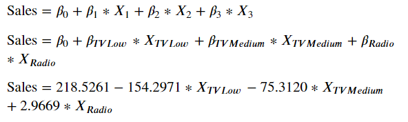
TV의 카테고리는 low, medium, high 3가지이다. 그런데 모델의 회귀계수를 보면 negative한 low, medium밖에 없는데 그 이유는 high 값이 default이기 때문이다.
3) p-value, 신뢰구간
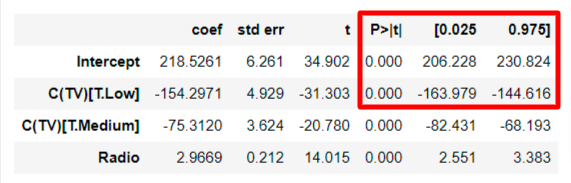
모든 회귀계수에 대한 p-value는 0.000으로 신뢰수준 5%에서 통계적으로 유의미하고, 95%에 해당하는 신뢰구간은 C(TV low)같은 경우 [-163.979, -144.616]에 해당한다.