pie chart
pie chart를 만들기 위해서는 split, apply, combine 과정을 거친다.
df_continents = df_can.groupby('Continent', axis=0).sum()
파이차트를 효과적으로 만들어줄 것들이 있다.
- autopct - is a string or function used to label the wedges with their numeric value. The label will be placed inside the wedge. If it is a format string, the label will be fmt%pct. - % 표시
- startangle - rotates the start of the pie chart by angle degrees counterclockwise from the x-axis. -시작각도
- shadow - Draws a shadow beneath the pie (to give a 3D feel).- 그림자
- legend - 범례추가
- pctdistance 파이차트 바깥에 %넣기
- color
- explode
# autopct create %, start angle represent starting point
df_continents['Total'].plot(kind='pie',
                            figsize=(5, 6),
                            autopct='%1.1f%%', # add in percentages
                            startangle=90,     # start angle 90° (Africa)
                            shadow=True,       # add shadow
                            )

plt.title('Immigration to Canada by Continent [1980 - 2013]')
plt.axis('equal') # Sets the pie chart to look like a circle.

plt.show()
colors_list = ['gold', 'yellowgreen', 'lightcoral', 'lightskyblue', 'lightgreen', 'pink']
explode_list = [0.1, 0, 0, 0, 0.1, 0.1] # ratio for each continent with which to offset each wedge.

df_continents['Total'].plot(kind='pie',
                            figsize=(15, 6),
                            autopct='%1.1f%%',
                            startangle=90,
                            shadow=True,
                            labels=None,         # turn off labels on pie chart
                            pctdistance=1.12,    # the ratio between the center of each pie slice and the start of the text generated by autopct
                            colors=colors_list,  # add custom colors
                            explode=explode_list # 'explode' lowest 3 continents
                            )

# scale the title up by 12% to match pctdistance
plt.title('Immigration to Canada by Continent [1980 - 2013]', y=1.12)

plt.axis('equal')

# add legend
plt.legend(labels=df_continents.index, loc='upper left')

plt.show()
box plots
# horizontal box plots
df_CI.plot(kind='box', figsize=(10, 7), color='blue', vert=False)

plt.title('Box plots of Immigrants from China and India (1980 - 2013)')
plt.xlabel('Number of Immigrants')

plt.show()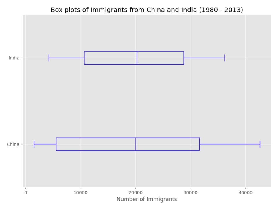
scatter plots
기본 산점도 plot이다.
df_tot.plot(kind='scatter', x='year', y='total', figsize=(10, 6), color='darkblue')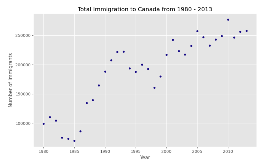
여기에 numpy의 polyfit() 함수를 써보자.
degree는 차수를 뜻한다.
polynomial적인 의미이다.
polyfit 함수로 학습을 하면 1차 함수의 a, x 값을 도출한다.
x = df_tot['year']      # year on x-axis
y = df_tot['total']     # total on y-axis
fit = np.polyfit(x, y, deg=1)
여기에 annotate를 달고, 직선을 그려보자.
plt.plot(x, fit[0] * x + fit[1], color='red') # recall that x is the Years
plt.annotate('y={0:.0f} x + {1:.0f}'.format(fit[0], fit[1]), xy=(2000, 150000))

plt.show()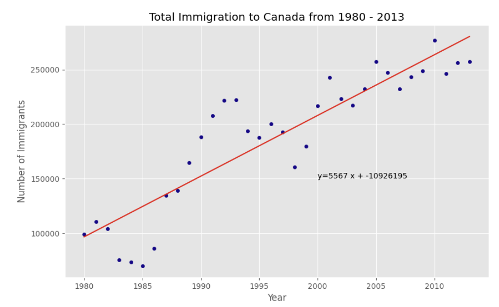
subplot
여러 개의 plot을 만들고 싶을 때 figure() 함수를 쓰는데, 여기는 artist layer이다.
전형적인 문장은
fig = plt.figure() #create figure
ax=fig.add_subplot(nrows, ncols, plot_number) #create sublot
nrows, ncols는 행과 열의 전체 개수를 뜻한다. nrows*ncols 가 subplot의 전체개수
plot number는 해당 플랏이 몇 번째 순서인지를 확인한다.
subplot(211)==subplot(2,1,1) 똑같은 의미이다.
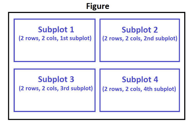
fig = plt.figure() # create figure

ax0 = fig.add_subplot(1, 2, 1) # add subplot 1 (1 row, 2 columns, first plot)
ax1 = fig.add_subplot(1, 2, 2) # add subplot 2 (1 row, 2 columns, second plot). See tip below**

# Subplot 1: Box plot
df_CI.plot(kind='box', color='blue', vert=False, figsize=(20, 6), ax=ax0) # add to subplot 1
ax0.set_title('Box Plots of Immigrants from China and India (1980 - 2013)')
ax0.set_xlabel('Number of Immigrants')
ax0.set_ylabel('Countries')

# Subplot 2: Line plot
df_CI.plot(kind='line', figsize=(20, 6), ax=ax1) # add to subplot 2
ax1.set_title ('Line Plots of Immigrants from China and India (1980 - 2013)')
ax1.set_ylabel('Number of Immigrants')
ax1.set_xlabel('Years')

plt.show()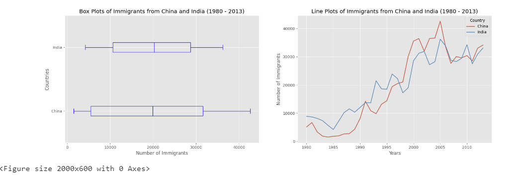
'Certificate > data science-IBM' 카테고리의 다른 글
| dashboard (0) | 2023.05.11 |
|---|---|
| waffle chart, word clouds, regplot, folium, choropleth maps (0) | 2023.05.10 |
| area plot, histogram, bar chart, annotate (0) | 2023.05.09 |
| data visualization with python, matplotlib architecture, %matplotlib inline (0) | 2023.05.05 |
| Model Evaluation, refinement, overfitting, underfiiting, grid search, hyperparameters, ridge regression, polynomial transform (0) | 2023.05.05 |