목차
로지스틱 회귀
1. What is logistic regression?
로지스틱 회귀는 범주화된 값들을 분류하는 알고리즘이다.
예컨데, 여러 요인들을 근거로 최종값이 어떤 범주에 속하는지 분류하는 것이다.
최종값 dependent variable을 산출해 내는데 필요한 것은 independent variables이다. 개수는 하나일 수도, 여러 개일 수도 있다. 다만 값은 연속적이어야 한다. 만약 범주형이라면 dummy형으로 변환하여 연속적인 값으로 바꾸어줘야 한다. 반면, dependant variable은 categorical한 값이다. binary할 수도 있고, multiple할 수 있다. 예컨데, 성공하거나 성공하지 않는다. true/false, 클래스 a, b, c 중 하나에 속한다 등이 있다. 최종적으로 특정 클래스에 속할 확률을 구해서, predict한다.
로지스틱 회귀는 가중치변수가 선형이므로 선형 회귀(linear regression) 계열은 맞다. 하지만, 학습으로 최적 회귀선을 찾는 일반 회귀모델과는 달리, '시그모이드 함수'의 최적선을 찾고 이 시그모이드 함수의 반환 값을 확률로 간주하고, 이에 따라 분류를 결정한다는 것이 다르다.
만약 categorical한 값을 찾는 문제에서 linear regression 모델을 도입하면 제대로 된 결과가 나오지 않을 것이다.
2. In which situations do we use logistic regression?
- 결괏값에 영향을 끼치는 변수를 알고 싶을 때
- target 데이터가 binary할 때
- 결괏값으로 확률을 도출하고 싶을 때
- data들이 특정 선형 함수로 분류될 때


3. 수학적으로 표현해보자.
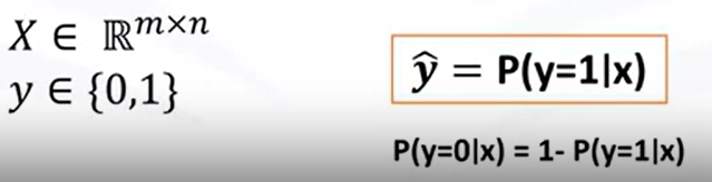
X 는 independent variable로 m*n의 값으로 구성된다.
Y는 dependent variable로 0 또는 1의 값을 취한다.
Yhat은 예측값으로 x가 1일 확률이다.
4. sigmoid function = logistic function
step function(임계치를 넘느냐의 여부에 따라 함수값이 결정되는)와 닮았다.
하지만 딱딱 끊기는 계단함수와는 달리 시그모이드는 부드로운 곡선형태이다.
시그모이드는 활성함수로서, 계산된 값을 시그모이드 함수에 넣으면 값을 0~1사이로 변환해서 출력한다.
아래의 수식을 보자
exponential 값이 커질 수록 값은 1에 가까워진다.
반대로 값이 작을 수록 값은 0에 가까워진다.
이는 확률값으로 본다.
0<=sigmoid함수값<=1


ex) P(class=1|소득, 나이)=0.3
P(class=0|소득, 나이) = 1- P(class=1|소득, 나이)= 0.7
5. 모델 만드는 과정
1) initialize thetas(random value)

2) calculate y hat= sigmoid(transpose theta X) ---->probability
3) calculate all error-----> use cost function---> lower cost, better model


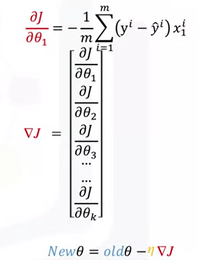
4) calculate the gradient of cost function

5) change the theta to reduce the cost-----> minimize the cost function value--->update weights with new values

6) go back to step 2
iteration: accuracy가 만족할 만한 값에 도달하면 횟수를 멈춘다.
theta값을 바꾸는 기준? 다양하지만, 대체로 gradient descent를 사용한다.
learning rate를 조정하여 학습의 속도를 조절한다.
7) Predict the X!
7. optimize the model
1) how to find the best parameters for our model?- cost function
use cost function
(1) MSE
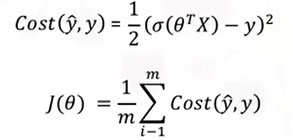
(2) CEE(Cross Entropy Error)
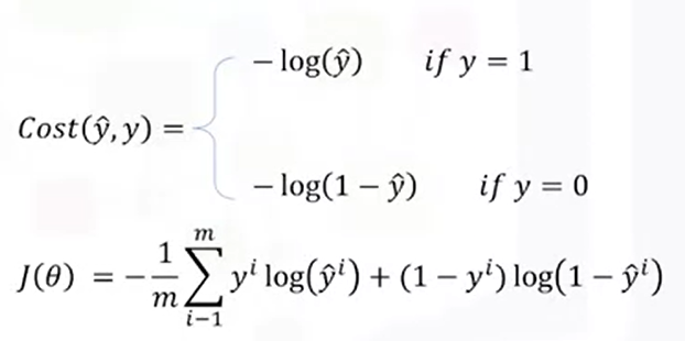
2) how to minimize the cost function? - gradient descent
- Gradient Descent 경사하강법
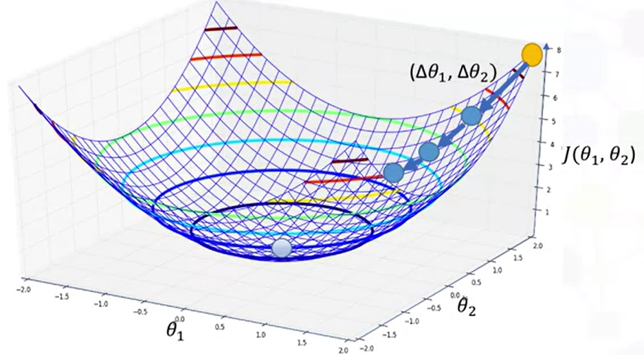
위 의 그래프는 세타1, 세타2 값에 따른 손실함수(cost function) 값을 나타냈다.
이 그래프를 통해 손실함수 값이 최소가 되는 지점의 파라미터 세타1, 세타2 값을 찾아보자.
파라미터 2개를 가지고 손실함수 값을 계산해봐야 할 것이다.
노란색 점을 start point로 랜덤하게 잡았다고 가정하고 한 걸음 내딛는다. 아직 최소점이 아니라면 또 한 걸음 내딛는다. 최소값에 도다를 때까지 말이다.
3) 가긴 가는데, 어떤 방향으로 갈 것인가?- learning rate
여기서 gradient 기울기가 나온다. 기울기는 x의 증가분에 y의 증가분으로서 uphill로 가는 방향이다.
이 원리를 생각하면, 기울기의 반대 방향으로 진행해야 된다는 것을 알 수 있다.
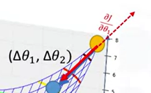
얼마나 큰 보폭으로 갈 것인가?
학습률이라고 한다. 학습률을 조금씩 임의로 변경해보며 모델을 튜닝한다.
import pandas as pd
import pylab as pl
import numpy as np
import scipy.optimize as opt
from sklearn import preprocessing
%matplotlib inline
import matplotlib.pyplot as plt

#data 가져오기
churn_df = pd.read_csv(path)
churn_df.head()

#data exploratory
churn_df.shape

#data를 X, y set으로 바꾸고 numpy 배열로 바꾸기
X = np.asarray(churn_df[['tenure', 'age', 'address', 'income', 'ed', 'employ', 'equip']])
X[0:5]
y = np.asarray(churn_df['churn'])
y [0:5]

#data normalization
from sklearn import preprocessing
X = preprocessing.StandardScaler().fit(X).transform(X)
X[0:5]

#train/test split, random_state=4(데이터셋 바뀌지 않도록)
from sklearn.model_selection import train_test_split
X_train, X_test, y_train, y_test = train_test_split( X, y, test_size=0.2, random_state=4)
print ('Train set:', X_train.shape,  y_train.shape)
print ('Test set:', X_test.shape,  y_test.shape)

#모델링
from sklearn.linear_model import LogisticRegression
from sklearn.metrics import confusion_matrix
LR = LogisticRegression(C=0.01, solver='liblinear').fit(X_train,y_train)
LR2= LogisticRegression(C=0.01, solver='sag').fit(X_train, y_train)
LR

#예측값
yhat = LR.predict(X_test)
yhat

#예측확률(a, b)
yhat_prob = LR.predict_proba(X_test)
yhat_prob

#evaluation - jaccard index(intersection 비율)
from sklearn.metrics import jaccard_score
jaccard_score(y_test, yhat,pos_label=0)

#evaluation - accuracy of confusion matrix
from sklearn.metrics import classification_report, confusion_matrix
print(confusion_matrix(y_test, yhat, labels=[1,0]))

# visualization -confusion matrix
import itertools
def plot_confusion_matrix(cm, classes,
                          normalize=False,
                          title='Confusion matrix',
                          cmap=plt.cm.Blues):
    """
    This function prints and plots the confusion matrix.
    Normalization can be applied by setting `normalize=True`.
    """
    if normalize:
        cm = cm.astype('float') / cm.sum(axis=1)[:, np.newaxis]
        print("Normalized confusion matrix")
    else:
        print('Confusion matrix, without normalization')

    print(cm)

    plt.imshow(cm, interpolation='nearest', cmap=cmap)
    plt.title(title)
    plt.colorbar()
    tick_marks = np.arange(len(classes))
    plt.xticks(tick_marks, classes, rotation=45)
    plt.yticks(tick_marks, classes)

    fmt = '.2f' if normalize else 'd'
    thresh = cm.max() / 2.
    for i, j in itertools.product(range(cm.shape[0]), range(cm.shape[1])):
        plt.text(j, i, format(cm[i, j], fmt),
                 horizontalalignment="center",
                 color="white" if cm[i, j] > thresh else "black")

    plt.tight_layout()
    plt.ylabel('True label')
    plt.xlabel('Predicted label')

np.set_printoptions(precision=2)

plt.figure()
plot_confusion_matrix(cnf_matrix, classes=['churn=1','churn=0'],normalize= False,  title='Confusion matrix')

print (classification_report(y_test, yhat))


#evaluation- log loss
from sklearn.metrics import log_loss
log_loss(y_test, yhat_prob)
LR2= LogisticRegression(C=0.01, solver='sag').fit(X_train, y_train)
1) optimizer : 'newton-cg’, ‘lbfgs’, ‘liblinear’, ‘sag’, ‘saga’ solvers
Newton-Conjugate Gradient ('newton-cg'): 이 해결자는 Newton's method와 공액 그래디언트를 결합합니다. 비용 함수의 헤시안 행렬(2차 도함수)을 근사화하고 수렴할 때까지 가중치를 반복적으로 업데이트합니다.
Limited-memory Broyden-Fletcher-Goldfarb-Shanno ('lbfgs'): LBFGS는 제한된 메모리를 사용하여 헤시안 행렬을 근사화하는 준-뉴턴 최적화 방법입니다. 많은 수의 특성을 가진 문제에 잘 작동합니다.
Liblinear: 이 해결자는 선형 모델에 특화되어 있으며, 선형 서포트 벡터 머신(SVM)을 기반으로 합니다. 좌표 하강 알고리즘을 사용하며 L1 및 L2 정규화를 지원합니다.
Stochastic Average Gradient ('sag'): SAG는 확률적 평균 그래디언트 방법으로, 비용 함수의 그래디언트의 근사치를 사용하여 가중치를 업데이트합니다. 대규모 데이터셋에 적합한 방법입니다.
Stochastic Average Gradient ('saga'): SAGA는 SAG의 변형으로, 각 특성에 대해 정규화(regularization)를 적용할 수 있는 기능을 제공합니다. 따라서 L1 및 L2 정규화를 지원하는 선형 모델에 사용됩니다.
2)C: regularization
C는 로지스틱 회귀(Logistic Regression) 모델에서 정규화(regularization) 강도를 조절하는 매개변수입니다. 정규화는 모델의 복잡성을 제어하여 과적합을 방지하고 일반화 성능을 향상시키는데 사용됩니다.
C의 값은 양의 실수로 설정되며, 값이 작을수록 정규화의 강도가 커집니다. 따라서 C가 작을수록 모델은 간단해지고, 큰 가중치 값에 패널티를 부여하여 모델의 일반화를 도모합니다.
예를 들어, LogisticRegression(C=0.01, solver='sag')에서 C 값이 0.01로 설정되어 있다면, 해당 모델은 상대적으로 강한 정규화를 가지게 됩니다. C 값이 작기 때문에 모델은 단순화되고, 작은 가중치 값에 더 큰 패널티를 부여하여 모델의 복잡성을 제한하려고 합니다.
C 값은 문제의 특성과 데이터셋에 따라 조정해야 합니다. 너무 큰 C 값은 과적합의 가능성을 높일 수 있고, 너무 작은 C 값은 모델의 표현력을 제한할 수 있습니다. 적절한 C 값을 선택하기 위해서는 교차 검증(cross-validation) 등의 기법을 활용하여 모델의 성능을 평가하고 최적의 C 값을 찾는 것이 일반적입니다.
8. Softmax
만약 최종 분류값이 multiple하다면 활성화함수로 softmax를 사용하는 것이 좋다.
lr = LogisticRegression(random_state=0).fit(X, y)
probability=lr.predict_proba(X)
np.argmax(probability[0,:])
softmax_prediction=np.argmax(probability,axis=1)
yhat =lr.predict(X)
accuracy_score(yhat,softmax_prediction)
'머신러닝 > machine learning' 카테고리의 다른 글
| clustering, k-means (1) | 2023.05.18 |
|---|---|
| classification, SVM, support vector machine, kerneling (0) | 2023.05.18 |
| classification, regression tree (0) | 2023.05.18 |
| classification, decision tree, entropy, 지니계수, information gain (0) | 2023.05.17 |
| classification, KKN(k-nearest neighbors), evaluate metrics, f1 score, log loss, Jaccard index (0) | 2023.05.17 |