목차
SVM support vector machine
지도학습으로 separator을 찾아서 여러 케이스들을 분류하는 것이다.
SVM은 데이터를 고차원 공간으로 맵핑한 후, separator을 찾는다.
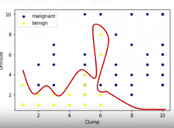
아래와 같이 2차원 공간에 데이터를 두면, linear하게 separate 되지 않는다.
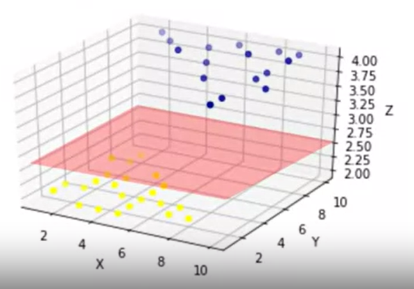
그런데 만약 아래와 같이 고차원 공간에 피처들을 놓는다면, 이야기가 달라진다.
데이터들이 고차원평면으로 separte된다.
SVM은 데이터를 분류할 수 있는 최적의 고차원평면(hyperplane)을 찾는 것이 목적이다.
Kerneling
SVM 알고리즘에서는 kernel 함수 옵션을 제공한다. 고차원 공간으로 데이터를 매핑시키는 것을 커널링이라고 한다. 커널링은 수학적인 함수이며, 다양한 타입이 있다. 모두 장점과 단점이 다르므로 데이터셋의 특징에 맞게 가져와서 쓴다.
Linear, Polynomial, Radial basis function(RBF), Sigmoid
장점과 단점
장점: 고차원 공간에서 정확하고, 메모리 공간이 효율적이다.
단점: 오버피팅의 가능성이 높고, 확률을 제공하지 않고, 데이터세트가 너무 큰 경우 계산 효율성이 높지 않다.
언제 SVM을 쓰는가?
결론적으로 (high demensional data)에 쓰기가 좋다.
예컨데,
image recognition
text mining
ex) text category assignment , detecting spam, sentiment analysis 스팸 탐지, 감정분석
gene expression classification
import pandas as pd
import pylab as pl
import numpy as np
import scipy.optimize as opt
from sklearn import preprocessing
from sklearn.model_selection import train_test_split
%matplotlib inline
import matplotlib.pyplot as plt

cell_df = pd.read_csv("cell_samples.csv")
cell_df.head()

#data exploratory- visualization
ax = cell_df[cell_df['Class'] == 4][0:50].plot(kind='scatter', x='Clump', y='UnifSize', color='DarkBlue', label='malignant');
cell_df[cell_df['Class'] == 2][0:50].plot(kind='scatter', x='Clump', y='UnifSize', color='Yellow', label='benign', ax=ax);
plt.show()

#data preprocessing
cell_df.dtypes

#object type의 feature을 int type으로 변환
cell_df = cell_df[pd.to_numeric(cell_df['BareNuc'], errors='coerce').notnull()]
cell_df['BareNuc'] = cell_df['BareNuc'].astype('int')
cell_df.dtypes

#X, y 저장하고, numpy배열로 바꾸기
feature_df = cell_df[['Clump', 'UnifSize', 'UnifShape', 'MargAdh', 'SingEpiSize', 'BareNuc', 'BlandChrom', 'NormNucl', 'Mit']]
X = np.asarray(feature_df)
X[0:5]

cell_df['Class'] = cell_df['Class'].astype('int')
y = np.asarray(cell_df['Class'])
y [0:5]

#train/test split
X_train, X_test, y_train, y_test = train_test_split( X, y, test_size=0.2, random_state=4)
print ('Train set:', X_train.shape,  y_train.shape)
print ('Test set:', X_test.shape,  y_test.shape)

#SVM modeling -kerneling: 'rbf'
from sklearn import svm
clf = svm.SVC(kernel='rbf')
clf.fit(X_train, y_train)

# prediction
yhat = clf.predict(X_test)
yhat [0:5]

#evaluation- confusion_matrix
from sklearn.metrics import classification_report, confusion_matrix
cnf_matrix = confusion_matrix(y_test, yhat, labels=[2,4])
np.set_printoptions(precision=2)
print (classification_report(y_test, yhat))

# visualization
import itertools
def plot_confusion_matrix(cm, classes,
                          normalize=False,
                          title='Confusion matrix',
                          cmap=plt.cm.Blues):
    """
    This function prints and plots the confusion matrix.
    Normalization can be applied by setting `normalize=True`.
    """
    if normalize:
        cm = cm.astype('float') / cm.sum(axis=1)[:, np.newaxis]
        print("Normalized confusion matrix")
    else:
        print('Confusion matrix, without normalization')

    print(cm)

    plt.imshow(cm, interpolation='nearest', cmap=cmap)
    plt.title(title)
    plt.colorbar()
    tick_marks = np.arange(len(classes))
    plt.xticks(tick_marks, classes, rotation=45)
    plt.yticks(tick_marks, classes)

    fmt = '.2f' if normalize else 'd'
    thresh = cm.max() / 2.
    for i, j in itertools.product(range(cm.shape[0]), range(cm.shape[1])):
        plt.text(j, i, format(cm[i, j], fmt),
                 horizontalalignment="center",
                 color="white" if cm[i, j] > thresh else "black")

    plt.tight_layout()
    plt.ylabel('True label')
    plt.xlabel('Predicted label')

plt.figure()
plot_confusion_matrix(cnf_matrix, classes=['Benign(2)','Malignant(4)'],normalize= False,  title='Confusion matrix')

# evaluation - F1_score
from sklearn.metrics import f1_score
f1_score(y_test, yhat, average='weighted')

# evaluation -Jaccard index
from sklearn.metrics import jaccard_score
jaccard_score(y_test, yhat,pos_label=2)'머신러닝 > machine learning' 카테고리의 다른 글
| 머신러닝 과정 전체, preprocessing.StandardScaler(), fit(), transform(), fit_transform(), gridsearchCV, scores (0) | 2023.06.03 |
|---|---|
| clustering, k-means (1) | 2023.05.18 |
| logistic regression, sigmoid, logistic regression vs linear regression, C, optimizer, softmax (0) | 2023.05.18 |
| classification, regression tree (0) | 2023.05.18 |
| classification, decision tree, entropy, 지니계수, information gain (0) | 2023.05.17 |