12차시 다항 회귀 polynomial Regression, subplot, 차원, plt.setp, polynomialfeatures, 시각화, tradeoff, overfit, 규제화, regularization, ridge, lasso, elasticnet, concatenate, pd.concat, reset

Kaggle

12차시 다항 회귀 polynomial Regression, subplot, 차원, plt.setp, polynomialfeatures, 시각화, tradeoff, overfit, 규제화, regularization, ridge, lasso, elasticnet, concatenate, pd.concat, reset_index()

Olivia-BlackCherry 2024. 4. 26. 06:48

다항회귀 ?

데이터가 단순한 직선형태가 아니라 비선형의 형태일 때, 각 독립변수의 거듭제곱을 새로운 변수로 추가하면 선형 모델을 사용할 수 있다. 즉, 독립변수가를단항식이 아닌 2차, 3차 방정식과 같은 다항식으로 표현됨.

단, 독립변수는 비선형 형태가 되지만 다항회귀 자체는 여전히 선형회귀이다. 회귀계수가 여전히 선형이기 때문이다.

ex) 나이에 따른 보험가격에 대한 회귀선 ---> 나이(X)를 거듭제곱하여 새로운 독립변수로 만듬

< python code 1 >

# train/test data split
from sklearn.model_selection import train_test_split
x_train, x_test, y_train, y_test = train_test_split(x,y, test_size=0.3, random_state=156)

1. Polynomial 변환

X변수 > 다항식(Polynomial)으로 변환

♡ 예제 데이터

# Polynomial Feature 만들기
from sklearn.preprocessing import PolynomialFeatures
import numpy as np

# 단항식 예제 만들기
X = np.arange(4).reshape(2,2)
print(X)
# x1=0, x2=1
# X3=2, x4=3

[[0 1]
 [2 3]]

♡ 2차 다항식

# 2차 다항식으로 변환 
poly = PolynomialFeatures(degree=2)
poly.fit(X)
poly_ftr = poly.transform(X)
print(poly_ftr)
# 1, x1=0, x2=1, x1의제곱=0, x1*x2=0, x2의제곱=1
# 1, x3=2, x4=3, x3의제곱=4, x3*x4=6, x4의제곱=9

[[1. 0. 1. 0. 0. 1.]
 [1. 2. 3. 4. 6. 9.]]

♡ 3차 다항식

# 3차 다항식 변환
poly = PolynomialFeatures(degree=3)
poly_ftr = poly.fit_transform(x_train)
print("3차다항식계수", poly_ftr)

3차다항식계수 [[1.00000e+00 2.80000e+01 7.84000e+02 2.19520e+04]
 [1.00000e+00 1.80000e+01 3.24000e+02 5.83200e+03]
 [1.00000e+00 2.30000e+01 5.29000e+02 1.21670e+04]
 ...
 [1.00000e+00 6.10000e+01 3.72100e+03 2.26981e+05]
 [1.00000e+00 3.30000e+01 1.08900e+03 3.59370e+04]
 [1.00000e+00 4.90000e+01 2.40100e+03 1.17649e+05]]

2. 회귀모델 만들기

# LinearRegression 모델 만들기
lr= LinearRegression()
model = lr.fit(poly_ftr, y_train)
print(np.round(model.coef_))
print(np.round(model.intercept_))

[  0. 136.   0.   0.]
5885.0

--> 다항계수가 늘어남

model.coef_.shape

# (4,0)

3. x_test 역시 다항식으로 변환

♡ 배열 형태 바꾸기

- 많은 머신러닝 모델들이 2차원 배열 형태의 입력을 요구한다.

- 배열 간 연산을 수행할 때 차원이 일치해야 한다.

X_test= X_test.reshape(행, 1)

y_test = np.array(y_test)

x_test = x_test[:, np.newaxis]

♡ fit()하지 않고, transform만!

x_test_poly = poly.transform(x_test)
pred= model.predict(x_test_poly)
np.round(pred[:3],2)

array([18189.37,  8754.09, 15727.4 ])

4. 평가

♡ mse, rmse 회귀 평가지표 사용하기

#평가
from sklearn.metrics import mean_squared_error, r2_score
mse = mean_squared_error(y_test, y_pred)
rmse = np.sqrt(mse)
r2score= r2_score(y_test, y_pred)
print("MSE:{0:.3f}, RMSE: {1:.3f}".format(mse, rmse))
print("R2 Score:{:.3f}".format(r2score))

MSE:123272344.532, RMSE: 11102.808
R2 Score:0.046

<python code 2>

1. 예제 데이터 만들기

import numpy as np
import matplotlib.pyplot as plt
from sklearn.preprocessing import PolynomialFeatures
from sklearn.linear_model import LinearRegression
from sklearn.model_selection import cross_val_score

# 예제 데이터 만들기
def true_fun(X):
    return np.cos(1.5*np.pi*X)

# 0~1까지 30개의 임의 값을 순서대로 샘플링하기
np.random.seed(0)
n_samples = 30
X= np.sort(np.random.rand(n_samples))

# y값은 코사인 기반 true_fun()에 노이즈값을 더함
y= true_fun(X) + np.random.randn(n_samples)*0.1

print(X, X.shape)
print(y, y.shape)

[0.02 0.07 0.09 0.12 0.14 0.38 0.41 0.42 0.44 0.46 0.52 0.53 0.54 0.55
 0.57 0.6  0.64 0.65 0.72 0.78 0.78 0.79 0.8  0.83 0.87 0.89 0.93 0.94
 0.96 0.98] (30,)
[ 1.08  0.87  1.14  0.7   0.78 -0.25 -0.22 -0.27 -0.46 -0.53 -0.86 -0.99
 -0.87 -0.83 -0.77 -0.83 -1.03 -1.03 -1.08 -1.01 -1.03 -0.64 -0.86 -0.75
 -0.7  -0.41 -0.5  -0.28 -0.26 -0.06] (30,)

2. 배열 바꾸기

X = X.reshape(30,1)
y= y.reshape(30,1)

3. X --> Polynomial 변환

 # X--> polynomial 변환 시작
polynomial_feature = PolynomialFeatures(degree=3, include_bias=False)
linear_regression = LinearRegression()
poly_ftr= polynomial_feature.fit_transform(X)
model = linear_regression.fit(poly_ftr, y)
print()
print("degree: ", 3, "차", " 회귀계수", model.coef_)

4. 교차검증

1) scoring: neg_mean_squared_error

MSE score

# 교차 검증으로 다항 회귀 평가
# 교차 검증에서 polynomial 변환된 x값 넣기
neg_scores= cross_val_score(model, poly_ftr, y, scoring="neg_mean_squared_error", cv=5)
print("개별 negative cross validation score: ", neg_scores)
mse_score = -1*np.mean(neg_scores)
print("MSE score: ", mse_score)

개별 negative cross validation score:  [-2.73 -0.24 -0.36 -0.1  -1.57]
MSE score:  1.0025079017604521

2) scoring: r2

MSE score

scores = cross_val_score(model, poly_ftr, y, scoring="r2", cv=5)
print('Cross-validation scores:', -1*scores)
print('Mean cross-validation score:', -1*scores.mean())

Cross-validation scores: [11.78  1.95 36.18  2.86 37.66]
Mean cross-validation score: 18.08638912466492

5. X test 배열 바꾸기

# test 데이터 만들기
X_test = np.linspace(0,1,100)
X_test[:3]

array([0.  , 0.01, 0.02])

# X_test 배열바꾸기
X_test= X_test[:, np.newaxis]
X_test[:3]

array([[[0.  ]],

       [[0.01]],

       [[0.02]]])

6. X_test --> Polynomial

# Xtest-->Polynomial
poly_X_test= polynomial_feature.transform(X_test)
poly_X_test[:3]

array([[31.45],
       [10.19],
       [ 1.09]])

7. 시각화까지

1) 그래프 바탕 만들기( subplot)

♡ plt.subplot(행, 열, subplot번호)

subplot은 하나의 큰 그림 안에 여러 개의 작은 그림을 배치하는 것이며, plot은 하나의 그림을 의미한다.

plt.figure(figsize=(14,5))
for i in range(len(degrees)):
    # subplot(행, 열, subplot번호)
    ax= plt.subplot(1, len(degrees), i+1)

▼

▽

    # x,y 눈금 제거
    plt.setp(ax, xticks=(), yticks=())

♡ subplots_adjust()

subplot 간 간격 조정하기

plt.subplots_adjust()

▼

▽

2) 다항식 시각화 시작!

import numpy as np
import matplotlib.pyplot as plt
from sklearn.preprocessing import PolynomialFeatures
from sklearn.linear_model import LinearRegression
from sklearn.model_selection import cross_val_score

# 예제 데이터 만들기
def true_fun(X):
    return np.cos(1.5*np.pi*X)

# 0~1까지 30개의 임의 값을 순서대로 샘플링하기
n_samples = 30
X= np.sort(np.random.rand(n_samples))

# y값은 코사인 기반 true_fun()에 노이즈값을 더함
y= true_fun(X) + np.random.randn(n_samples)*0.1

# 차원바꾸기
X = X.reshape(30,1)
y= y.reshape(30,1)
x.shape, y.shape

# 다항식 만들고, 차수를 1, 4, 15로 변경하기
plt.figure(figsize=(14,5))
degrees=[1,4,15]

for i in range(len(degrees)):
    # subplot(행, 열, subplot번호)
    ax= plt.subplot(1, len(degrees), i+1)
    # x,y 눈금 제거
    plt.setp(ax, xticks=(), yticks=())
    
    # degree별로 polynomial 변환 시작
    polynomial_feature = PolynomialFeatures(degree=degrees[i], include_bias=False)
    linear_regression = LinearRegression()
    poly_ftr= polynomial_feature.fit_transform(X)
    
    # 변환된 x, y 넣어 regression모델 만들기
    model = linear_regression.fit(poly_ftr, y)
    print()
    print("degree: ", degrees[i],"차", " 회귀계수", model.coef_)
    
    # 교차 검증으로 다항 회귀 평가
    # 교차 검증에서 polynomial 변환된 x값 넣기
    neg_scores= cross_val_score(model, poly_ftr, y, scoring="neg_mean_squared_error", cv=5)
    print("개별 negative cross validation score: ", neg_scores)
    mse_score = -1*np.mean(neg_scores)
    print("MSE score: ", mse_score)
    
    rmse_score = np.sqrt(-1*neg_scores)
    print("개별 rmse score: ", rmse_score)
    rmse_score = np.mean(rmse_score)
    print("평균 rmse score:", rmse_score)
    
    # test 데이터 만들기
    X_test = np.linspace(0,1,100)
    X_test= X_test[:, np.newaxis]
    poly_X_test= polynomial_feature.transform(X_test)
    
    #예측값 곡선
    plt.plot(X_test, model.predict(poly_X_test), label="Model")
    
    #실제값 곡선
    y_test= true_fun(X_test)
    plt.plot(X_test, y_test,'--', label="True Function")
#     plt.scatter(X_test, y_test, s=5, edgecolor='r', alpha=0.7, label="samples")
    
    # legend
    plt.legend(loc="best")
    
    #label
    plt.xlabel("x")
    plt.ylabel("y")
    plt.xlim(0,1)    
    # title
    plt.title("Degree{}".format(degrees[i]))

plt.show()

degree:  1 차  회귀계수 [[-1.58]]
개별 negative cross validation score:  [-1.76 -0.18 -0.47 -0.05 -1.4 ]
MSE score:  0.7711929905400632
개별 rmse score:  [1.33 0.42 0.68 0.22 1.18]
평균 rmse score: 0.7675122878202554

degree:  4 차  회귀계수 [[  0.76 -20.43  29.72 -11.2 ]]
개별 negative cross validation score:  [-3.07 -0.01 -0.01 -0.01 -0.36]
MSE score:  0.691134901561618
개별 rmse score:  [1.75 0.09 0.11 0.11 0.6 ]
평균 rmse score: 0.532181642912367

degree:  15 차  회귀계수 [[ 3.14e+02 -1.62e+04  3.89e+05 -5.05e+06  4.01e+07 -2.12e+08  7.82e+08
  -2.07e+09  3.97e+09 -5.57e+09  5.64e+09 -4.01e+09  1.90e+09 -5.40e+08
   6.94e+07]]
개별 negative cross validation score:  [-1.51e+14 -1.51e+01 -3.03e-01 -7.92e+00 -8.48e+06]
MSE score:  30227164912099.01
개별 rmse score:  [1.23e+07 3.88e+00 5.50e-01 2.82e+00 2.91e+03]
평균 rmse score: 2459330.059289339

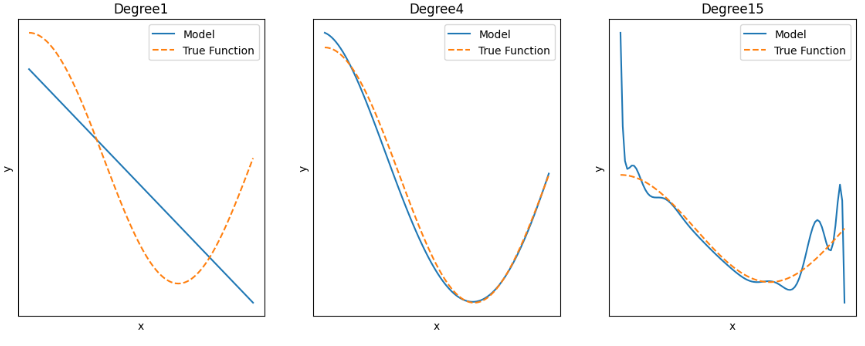
3) plot 그리기

- true function(노랑이점선): 실제값 곡선 (X_test, 함수(X_test))

- model(파랑이): 예측값 곡선 (X_test, y_pred)

- 범주, 타이틀, 라벨까지 붙이기

+ scatterplot 샘플 직접 나타내기

samples(빨강) : 원래, 실제 데이터 점--- 기본 true function에 노이즈있는 ---(X, y)

    plt.scatter(X, y, s=20, edgecolor='r', alpha=0.9, label="samples")

♡ alpha 투명도

♡ edgecolor r, g, b, c, m

♡ color r(red),g(green),b(blue),c(cyan:청록색),m(magenta:자홍색)

s 크기

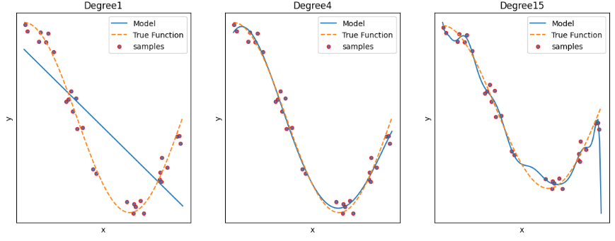
♡ 확대하기

xlim, ylim 이용

    plt.xlim(0,1)
    plt.ylim(-1, 1)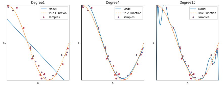

---> degree 1: 과소적합 / degree2: 적합 / degree3: 과대적합

Overfit

Rsquare은 모델이 데이터에 얼마나 적합한지 알 수 있다. 그런데 Rsquare가 너무 높은 것은 모델이 데이터에 과적합되어 있을 가능성이 높다. 과적합된 모델은 일반 다른 데이터에 대해 제대로 작동하지 못한다.

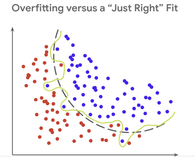
다항 회귀는 데이터의 복잡한 관계를 다항식으로 표현한다. 하지만 다항식의 차수(degree)가 높아질수록 매우 복잡한 피처 간의 관계까지 모델링이 가능해져서 오버피팅을 일으킬 수 있다. 오버피팅(과적합)이 발생하면 예측 정확도는 떨어진다.

결국, 좋은 예측 모델이란 학습 데이터의 패턴을 잘 반영하면서도 복잡하지 않은 균형잡힌 모델을 뜻한다.

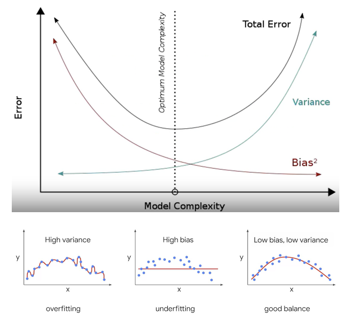
Bias - variance tradeoff

또한 좋은 모델은 편향과 분산 모두를 낮추는 것이다.

♡ degree1 : High Bias 고편향성 - 매우 단순한 모델로 지나치게 한 방향으로 치우친 경향을 보임

♡ degree4 : Low Bias, Low variance : 저편향, 저분산성 - 예측 결과가 실제와 근접하면서도 예측 변동이 크지 않고 특정 부분에 집중되어 뛰어난 성능을 보여줌.

♡ degree15 : High Variance 고분산성 - 매우 복잡한 모델로 지나치게 높은 변동성을 가짐

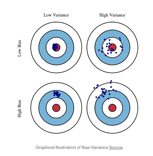
한쪽이 높으면 한쪽이 낮아지는 경향이 있는데, trade off 지점을 통과전후에 전체 오류 값이 증가한다. 따라서 편향과 분산이 서로 tradeoff를 이루며 전체 오류값이 낮아지는 모델을 구축하는 것이 가장 효율적이다.

Regularization( 규제화 )

Regularize regression
좋은 머신러닝 회귀 모델을 만들기 위해서는 비용함수(RSS)를 최소화하면서 회귀계수가 너무 커지지 않도록 해야 한다. 규제화(L1, L2, elastic)는 회귀식의 회귀계수 값에 패널티를 부여하면서 low bias가 되도록 예측성능을 조절한다.

< 예제 데이터 만들기 >

def true_fun(X):
    return np.cos(1.5*np.pi*X)

# 0~1까지 30개의 임의 값을 순서대로 샘플링하기
n_samples = 30
x= np.sort(np.random.rand(n_samples))

# y값은 코사인 기반 true_fun()에 노이즈값을 더함
y= true_fun(X) + np.random.randn(n_samples)*0.1

#차원
x= x.reshape(30,1)

규제화없는 데이터

평가

from sklearn.model_selection import cross_val_score
lr = LinearRegression()
neg_mse_scores = cross_val_score(lr, x, y, scoring="neg_mean_squared_error", cv=5)
print(mse_score)
mse_score = neg_mse_scores*(-1)
print("평균 교차검증 mse score", np.mean(mse_score))
rmse_score = np.sqrt(mse_score)
print("평균 교차검증 rmse score", np.mean(rmse_score))

[1.93 0.07 0.57 0.37 0.04]
평균 교차검증 mse score 0.8087238630821751
평균 교차검증 rmse score 0.8073840585468425

회귀계수

lr.fit(x,y).coef_[0]

array([-2.02])

1) Lasso (L1)

RSS(잔차제곱합) + 패널티항(절대값)

불필요한 회귀계수 급격히 감소시켜 0으로 만들고, 제거한다.

y변수를 예측하는데 크게 중요하지 않은 x변수를 제거한다.
유의미하지 않은 회귀계수를 0에 가깝게 만들기 때문에 변수 선택 효과가 있다.

from sklearn.linear_model import Lasso, ElasticNet

params= [0.01, 0.05, 0.1, 0.5, 1, 5]
for i, param in enumerate(params):
    # 다양한 alpha값
    lasso = Lasso(alpha=param)
    # 교차검정 평가 mse, rmse
    neg_mse_scores=cross_val_score(lasso, x, y, scoring="neg_mean_squared_error", cv=5)
    avg_rmse = np.mean(np.sqrt(-1*neg_mse_scores))
    print("avg_rmse: ", avg_rmse)
    # Lasso 학습 -> 회귀계수
    lasso.fit(x, y)
    coeff= lasso.coef_[i]
    print(param, " lasso_coeff: ", coeff)

avg_rmse:  0.7465390296439459
0.01  lasso_coeff:  [-1.77]
avg_rmse:  0.7253189292661888
0.05  lasso_coeff:  [-1.31]
avg_rmse:  0.7275829337170336
0.1  lasso_coeff:  [-0.73]
avg_rmse:  0.8279269585966105
0.5  lasso_coeff:  [-0.]
avg_rmse:  0.8279269585966105
1  lasso_coeff:  [-0.]
avg_rmse:  0.8279269585966105
5  lasso_coeff:  [-0.]

--> alpha의 값이 커지면서 일부 속성의 회귀계수가 0으로 바뀜. 회귀 계수가 0인 피처는 회귀 식에서 제외되며 변수 선택 효과를 낳는다.

2) Ridge (L2)

RSS(잔차제곱합) + 패널티항(제곱)

회귀계수의 크기를 감소시킨다.

y변수를 예측하는데 크게 중요하지 않은 x변수의 영향력을 최소화시킨다. (제거하지 X)
때문에 모든 x변수를 포함하고자할 때 좋다.
삭제하지 않기 때문에 변수 선택은 불가능하고, 변수 간 상관관계가 높은 상황에서 좋은 예측 성능을 발휘한다.

Ridge 규제화 적용--> 평가

from sklearn.linear_model import Ridge
from sklearn.model_selection import cross_val_score

# Ridge 모델 생성
ridge = Ridge(alpha=10)

# 교차 검증 수행
neg_mse_scores = cross_val_score(ridge, x, y, scoring="neg_mean_squared_error", cv=5)
print(mse_score)
mse_score = neg_mse_scores*(-1)
print("평균 교차검증 mse score", np.mean(mse_score))
rmse_score = np.sqrt(mse_score)
print("평균 교차검증 rmse score", np.mean(rmse_score))

[1.93 0.07 0.57 0.36 0.04]
평균 교차검증 mse score 0.5764310262681915
평균 교차검증 rmse score 0.6268075597494873

alpha 값 변화에 따른 평가값

alphas=[0,0.1,1,10,100]

for alpha in alphas:
    ridge = Ridge(alpha=alpha)
    
    # cross_val_score 이용해 5fold 의 평균 rmse 계산
    neg_mse_scores = cross_val_score(ridge, x, y, scoring="neg_mean_squared_error",cv=5)
    avg_rmse= np.mean(np.sqrt(-1*neg_mse_scores))
    print(alpha,": ", avg_rmse)

0 :  0.7535037947654935
0.1 :  0.7290046956257166
1 :  0.6492474775360726
10 :  0.7525755920419676
100 :  0.8189249139936294

줄어든 회귀계수

alphas=[0,0.1,1,10,100]

for i, alpha in enumerate(alphas):
    ridge = Ridge(alpha=alpha)
    # cross_val_score 이용해 5fold 의 평균 rmse 계산
    neg_mse_scores = cross_val_score(ridge, x, y, scoring="neg_mean_squared_error",cv=5)
    avg_rmse= np.mean(np.sqrt(-1*neg_mse_scores))
    print(alpha,": ", avg_rmse)
    
    # ridge 모델에 x,y 학습시킴
    ridge.fit(x, y)
    print(ridge.coef_[i])

0 :  0.7535037947654935
[-1.89]
0.1 :  0.7290046956257166
[-1.82]
1 :  0.6492474775360726
[-1.36]
10 :  0.7525755920419676
[-0.39]
100 :  0.8189249139936294
[-0.05]

3) ElasticNet

RSS(잔차제곱합) + alpha ( a*L1 +b*L2 )

대규모 데이터셋인 경우, 모델에서 변수를 없애야할지 말지 확실히 모르는 경우가 있다. 이럴 때 Elastic regression을 쓴다. L1+ L2 하이브리드형으로 상관관계가 큰 변수를 동시에 선택하고 배제하는 특성을 가진다.

엘라스틱넷은 alpha 값에 따라 회귀 계수변경하는 것을 완화하기 위해 L2 규제 추가함.

수행시간이 오래 걸림.

주요 파라미터

l1_ratio : a/ (a+b)

l1_ratio가 0이면 a가 0 ---> L2규제와 같음

l1_ratio 1이면 b가 0 ---> L1 규제와 같음.

from sklearn.linear_model import Lasso, ElasticNet
params= [0.01, 0.05, 0.1, 0.5, 1, 5]
for i, param in enumerate(params):
    # 다양한 alpha값
    elastic = ElasticNet(alpha=param, l1_ratio=0.7)
    
    # 교차검정 평가 mse, rmse
    neg_mse_scores=cross_val_score(elastic, x, y, scoring="neg_mean_squared_error", cv=5)
    avg_rmse = np.mean(np.sqrt(-1*neg_mse_scores))
    print("avg_rmse: ", avg_rmse)
    
    # elastic 학습 -> 회귀계수
    elastic.fit(x,y)
    coeff= elastic.coef_[i]
    print(param, "elasticNet:", coeff)

avg_rmse:  0.5604032789969855
0.01 elasticNet: [-1.88]
avg_rmse:  0.5848129310647783
0.05 elasticNet: [-1.4]
avg_rmse:  0.6370035591732414
0.1 elasticNet: [-0.93]
avg_rmse:  0.8279269585966105
0.5 elasticNet: [-0.]
avg_rmse:  0.8279269585966105
1 elasticNet: [-0.]
avg_rmse:  0.8279269585966105
5 elasticNet: [-0.]

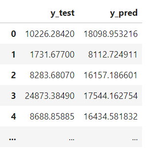
※ y_test, y_pred 비교하기

♡ concatenate()

#concatenate()함수
y_test = np.array(y_test)
np.concatenate((pred.reshape(len(pred),1), y_test.reshape(len(y_test),1)), axis=1)

array([[18189.37, 10226.28],
       [ 8754.09,  1731.68],
       [15727.4 ,  8283.68],
       [17447.46, 24873.38],
       [16056.55,  8688.86],

♡ pd.concat()

ytest_df = pd.DataFrame(y_test, columns=['y_test'])
ypred_df = pd.DataFrame(y_pred, columns=['y_pred'])
result = pd.concat([ytest_df, ypred_df], axis=1)
result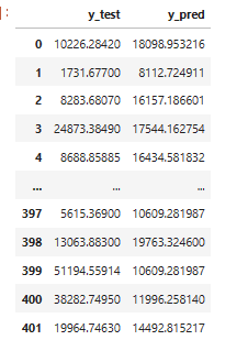

♡ reset_index(drop=True)

# DataFrame 만들기
ytest_df = pd.DataFrame(y_test, columns=['y_test'])
ypred_df = pd.DataFrame(y_pred, columns=['y_pred'])
result = pd.concat([ytest_df, ypred_df], axis=1)

# 인덱스 초기화
result.reset_index(drop=True)