목차
Logistic regression 로지스틱 회귀
A technique that models a categorical dependent variable Y based on one or more independent variables X
최고의 로지스틱 회귀 모델은?
The best logistic regression model estimates the set of beta coefficients that maximizes the likelihood of observing all of the sample data.
★ PACE - analyze
pace 과정 중에 data를 analyze하면서, 이 데이터에는 어떤 모델을 쓰는 것이 적합한지를 파악한다. 만약 이때 해당 데이터를 가지고 logisitc regression을 사용하고 싶다면, 아무런 근거 없이 결정해서는 안된다. 우선 logistic regression을 적용할 수 있다는 assumption을 설정하고, 해당 데이터가 그 가정을 침해하지 않은가를 확인해야 한다.
Binomial logistc regression
A technique that models the probability of an observation falling into one of two categories, based on one or more independent variables.
binary한 카테고리인 y variable을 사용한다.
Binomial logistic regression assumptions
1. ★ linearity
There should be a linear relationship between each X variable and the logit of the probability that Y equals 1.
1) odds
일어날 확률을 일어나지 않을 확률로 나눈 것

2) logit = log-odds
The logarithm of the odds of a given probability. So the logit of probability p is equal to the logarithm of p divided by 1minus p.

3) Logit in terms of X variables
X는 dependent variable에 영향을 미치는 independent x variables이다.

4) Maximum likelihood estimation(MLE)
A technique for estimating the beta parameters that maximize the likelihood of the model producing the observed data.
여기서 likelihood란 The probability of observing the actual data, given some set of beta parameters이다.
2. independent assumption

3. No muliticollinearity 다중공선성
4. No extreme outlier 아웃라이어 처리
★ PACE -construct
파이썬으로 logistic regression model을 만들어보자.
Python
사용데이터
accerlation에 따라, lying down의 값이 어떤 결과가 나오는가에 대한 데이터

1. 라이브러리
import pandas as pd
import seaborn as sns
from sklearn.model_selection import train_test_split
from sklearn.linear_model import LogisticRegression
2. X, y변수 정하기
X = activity[["Acc (vertical)"]]
y = activity[["LyingDown"]]
3. 데이터분할
X_train, X_test, y_train, y_test = train_test_split(X,y, test_size=0.3, random_state=42)
4. 모델 빌딩 및 학습
#clf는 classifier
clf = LogisticRegression().fit(X_train,y_train)
clf.coef_
clf.intercept_
회귀계수는?
array([[-0.1177466]])logistic regression coefficients report in percentages how much a factor increases or decreases the likelihood of an outcome.
y절편은?
array([6.10177895])
5. 그래프
sns.regplot(x="Acc (vertical)", y="LyingDown", data=activity, logistic=True)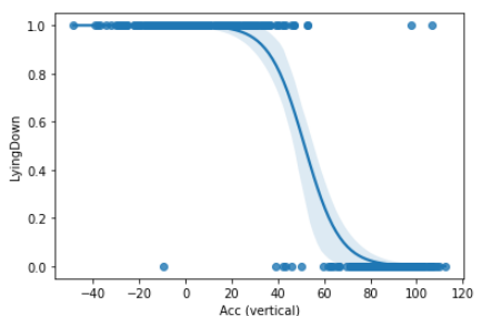
6. 예상값
y_pred = clf.predict(X_test)
y_pred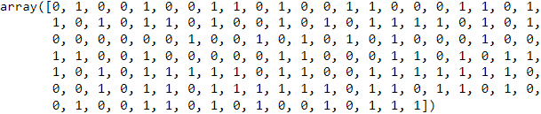
7. 예상 확률
clf.predict_proba(X_test)[::,-1]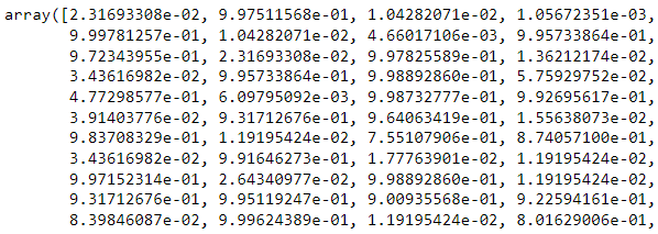
★ PACE: Analyze, Construct
모델에 대한 평가
evaluate
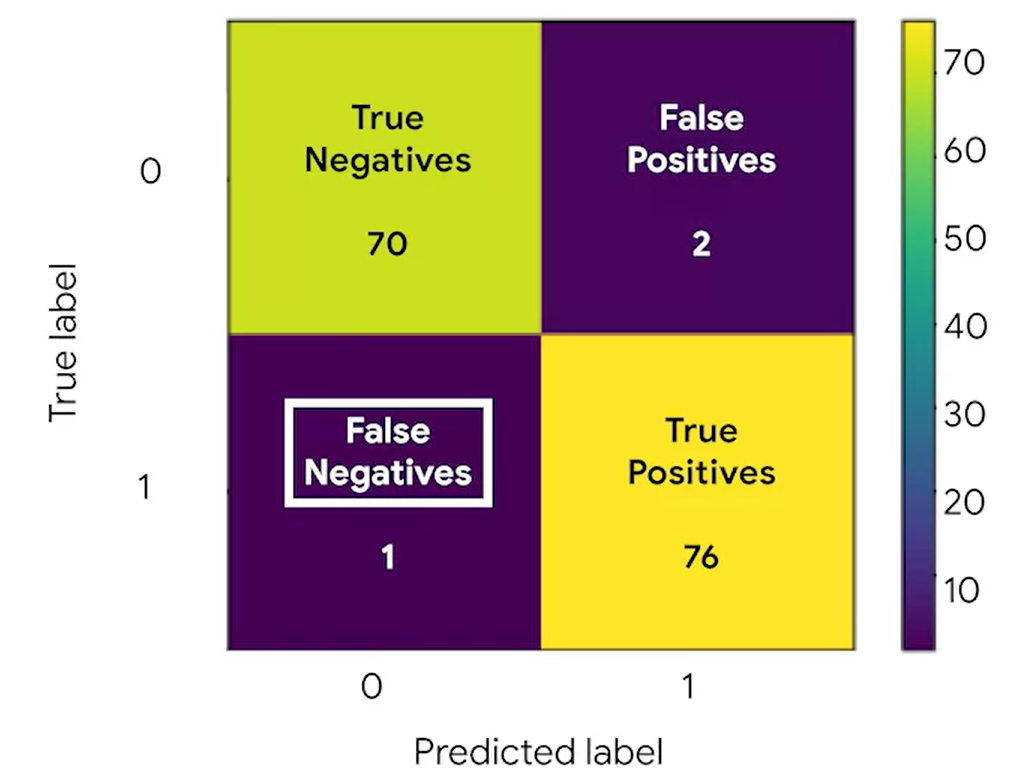
1. confusion matrix
A graphical representation of how accurate a classifer is at predicting the labels for a categorical variable.
혼동행렬로 이 모델이 성과가 괜찮은지 확인한다.
1) 라이브러리 호출
import sklearn.metrics as metrics
2) confusion matrix 출력(숫자만)
cm = metrics.confusion_matrix(y_test, y_pred, labels = clf.classes_)array([[70, 2],
[ 1, 76]])
3) 그래프로 출력
disp = metrics.ConfusionMatrixDisplay(confusion_matrix = cm,display_labels = clf.classes_)
disp.plot()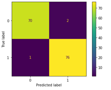
4) 해석
★ Precision

metrics.precision_Score(y_test, y_pred)
★ Recall

metrics.recall_Score(y_test, y_pred)
★ Accuracy

metrics.accuracy_score(y_test, y_pred)
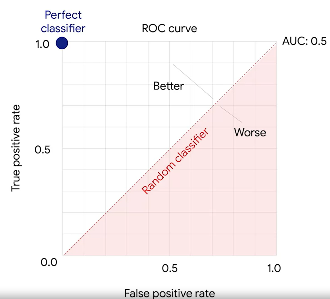
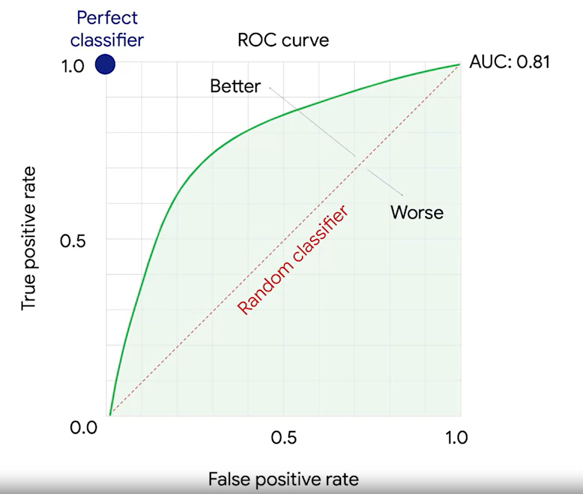
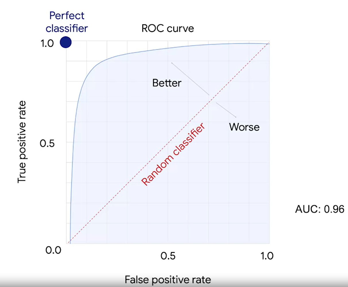
2. ROC curv, AUC
threshold에 따라서 혼동행렬 값이 달라진다.
ROC curve는 threshold에 따라 달라지는 TP와 FP의 비율을 곡선으로 보여준다.
AUC는 넓이다.
3. P-value
4. AIC, BIC