목차
Boosting
여러 개의 분류기가 순차적으로 학습을 수행하되, 앞에서 학습한 분류기가 예측이 틀린 데이터에 대해서 다음 분류기에 가중치를 부여하며 학습과 예측을 진행한다. 현재 성능이 매우 좋아 많은 산업에서 쓰이고 있으며 캐글 대회에서도 우수한 성적을 거두고 있는 방법이다.
Technique that builds an ensemble of weak learners sequentially, with each consecutive base learner trying to correct the errors of the one before.
< randomforest와 비교>
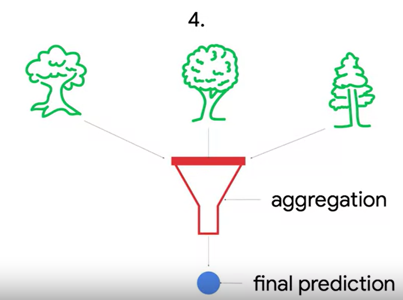
1. 같은 점
- ensembling technique
- Aggregates weak learners
2. 다른 점
- learners are built sequentially, not in parallel
부스팅에서는 전의 learner가 틀린 것이 무엇인지 집중해서 이를 개선하려 하기 때문에 연속적인 특성이 있다.
- not limited to tree-based learners
트리 베이스에만 국한되지 않는다.
< 종류>
1. Adaptive boosting(AdaBoost)
A boosting methodology where each consecutive base learner assigns greater weight to the observations incorrectly predicted by the preceding learner.


- 단점은 순서대로 진행해야하기 때문에 시간이 오래 걸린다.
- 정확도가 높다.
- 데이터를 스케일링하거나 정규화할 필요가 없다.
- numeric, categorical feature에 모두 적용된다.
-다중공선성 문제에도 크게 영향 받지 않는다.
- 이상치에도 큰 영향을 받지 않는다.
2. Gradient boosting
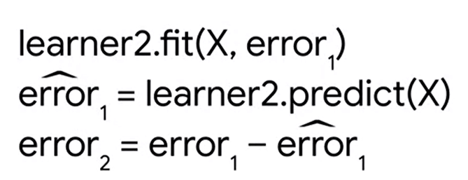
A boosting methodology where each base learner in the sequence is built to predict the residual errors of the model that preceded it.
앞선 AdaBoost와 비슷하나, 가중치 업데이트를 경사 하강법을 이용한다. error는 실제값-예측값이다.
error= y(실제값) - y^(예측값)
error를 최소화하는 방향으로 가중치값을 업데이트 해나가는 것이다.


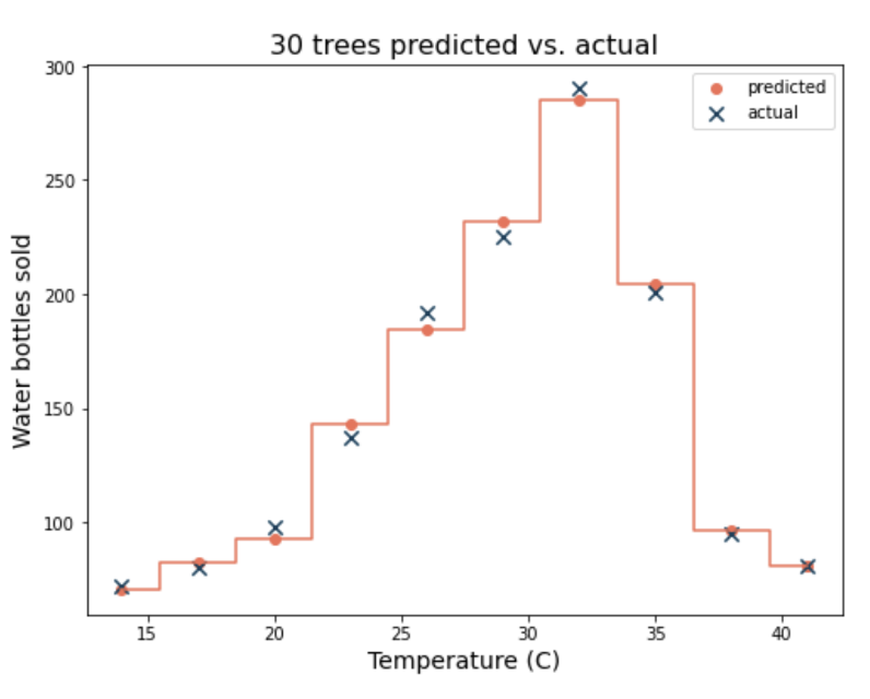
ex)

Gradient Boosting 모델로 학습한 뒤, 첫 번째 예측값이다. 실제값과 비교하여 그래프를 그려보자.

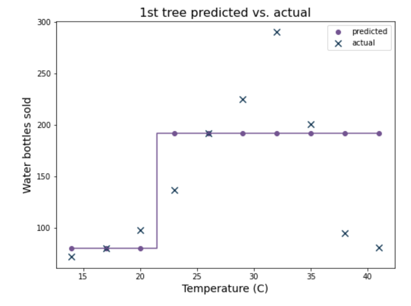
두 번째 tree로 학습한다. 두 번째를 학습할 때 X값은 그대로이지만, y값은 이전의 tree1 모델에서의 residual 즉 오차값이 된다. 최종 prediction은 tree1의 prediction값과 tree2의 prediction값을 더한 값이다. 즉 index 0 이라면 실제값은 72이지만, 첫번째 tree1에서의 prediction 80, 이에따른 오차인 -8이 두번째 tree에서의 y값이 되어 학습한 모델이 되고, 두 번째 prediction은 4.5이다. 따라서 최종 prediction은 80+4,5=84.5가 된다.

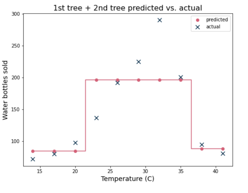
세 번째 tree로 학습한다. 세 번째 학습할 때의 y값은 이전 tree2 모델의 residual 값인 -8-4.5=-12.5가 되고, tree3의 prediction은 -4.5이다. 따라서 최종 prediction은 80+4.5-4.5=80이다.


만약 이것을 30개의 트리로 gradient boosting을 진행하면 마지막에는 실제값과 거의 유사하게 예측값이 나온다. decision tree일 때보다 훨씬 정확도가 높지만, 오버피팅의 우려도 커진다.
3. Gradient boosting machines
Model ensembles that use gradient boosting
<장점>
- 높은 정확도 high accuracy
- generally scalable 큰 규모의 데이터를 다룰 수 있는 능력이다. GBM은 작은 규모의 데이터셋부터 큰 규모까지 처리할 수 있다. 아무리 데이터가 크더라도 비교적 높은 효율성과 성능이 유지된다.
- tree base이기 때문에 데이터를 스캐일할 필요가 없고, 이상값을 다루기가 쉽다.
- missing value가 있더라도 괜찮다.
<단점>
-하이퍼파라미터가 많고 이를 처리하는데 시간이 오래 걸린다.
- black-box model이다. 즉, 이해하고 해석하기가 어렵다.
black box model
Any model whose predictions cannot be precisely explained
- have difficulty with extrapolation
Extrapolation 외삽법
A model's ability to predict new values that fall outside of the range of values in the training data.
외삽법은 주어진 데이터 범위를 넘어서서 값을 추정하는 것이다. 간단히 말해, 학습한 데이터 패턴을 기반으로 학습한 모델에서, 데이터 범위를 넘어서는 새로운 값을 예측하는 것을 의미한다.
ex) 1개는 200원 2개는 400원이면 3개는 600원이라고 외삽법에 의해 값을 내릴 수 있다.
하지만 외삽법은 늘 정확하지 않다. 예측하려는 범위가 너무 멀거나 데이터 패턴이 극단적으로 변한다면 부정확하거나 불안정해지기 때문이다.
GBM의 경우 주로 입력된 데이터 범위에서 잘 작동하도록 하이퍼파라미터 튜닝으로 오버피팅될 가능성이 높아서, 데이터 범위를 넘어서는 예측인 경우 오류가 발생할 확률이 높다. 따라서 GBM의 경우 외삽이 발생하는 상황을 가능한 피하고 모델이 학습한 데이터 범위 내에서 예측하는 것이 좋다.
4. XGBOOst(eXtra Gradient Boost)
Extreme gradient boosting, an optimized GBM package
트리 기반의 앙상블 학습에서 가장 각광받는 알고리즘이다. XGBoost는 GBM에 기반하지만, GBM의 느린 속도와 규제 부재 등의 문제를 해결한 업그레이드 된 모델이다. 또한 병렬 학습이 가능해 속도가 빠르다. 조정할 수 있는 하이퍼파라미터가 많다.
learning_rate(shrinkage)
How much weight is given to each consecutive tree's prediction in the final ensemble
각 트리가 이전 트리의 오차를 얼마나 크게 반영하여 학습할지를 결정하는 파라미터이다. lr가 크면 이전 트리의 오차를 크게 반영하기에 이 모델이 빠르게 학습될 수 있지만, 수렴하지 못하고 발산할 가능성이 있다. 반대로 lr가 작으면 이전 트리의 오차를 작게 반영하여 모델이 안정적으로 수렴하지만, 학습이 느려질 수 있다.
min_child_weight
결정트리에서 min_sample과 유사하다. 각 트리의 리프 노드를 분할할 때 최소로 필요한 데이터 샘플 수 이다.
A tree will not split a node if it results in any child node with less weight thatn this value.
Regularization 파라미터이다. 만약 min_child_weight가 크기에 따라 트리의 깊이가 달라지기 때문이다.
0-1(percentage, ex 0.1=10% of training observation)
1+(equivalent to the number of child observation, ex10 means no child node could contain fewer than 10 observations )
| max_depth | n_estimators | learning_rate | min_child_weight |
| 2-10 | 50-500 | 0.01-0.3 | 0-1 1+ |
| 최적화된 수치를 찾기 위한 가장 좋은 방법은 교차검증이다. 트리가 깊어질 수록 오버피팅될 가능성이 높다. | 작은 데이터셋에서는 트리가 많을 수록 유리하지만, 많은 데이터셋에서는 트리가 적을 수록 유리하다. | 작은 학습률은 over-correction이나 over-fitting을 방지한다. | 규제 파라미터로, 값이 클 수록 underfit가 발생할 가능성이 높다. 작을 수록 모델이 더 복잡해져 overfitting의 가능성이 있다. |
5. Python
1. 라이브러리
import numpy as np
import pandas as pd

# This is the classifier
from xgboost import XGBClassifier

# This is the function that helps plot feature importance
from xgboost import plot_importance

from sklearn.model_selection import GridSearchCV, train_test_split
from sklearn.metrics import accuracy_score, precision_score, recall_score,\
f1_score, confusion_matrix, ConfusionMatrixDisplay, RocCurveDisplay

import matplotlib.pyplot as plt

# This displays all of the columns, preventing Juptyer from redacting them.
pd.set_option('display.max_columns', None)

# This module lets us save our models once we fit them.
import pickle
2. 데이터


3. feature engineering
-feature selection
# Drop useless and sensitive (Gender) cols
churn_df = df_original.drop(['RowNumber', 'CustomerId', 'Surname', 'Gender'],
                            axis=1)
- feature transformation
churn_df2 = pd.get_dummies(churn_df, drop_first='True')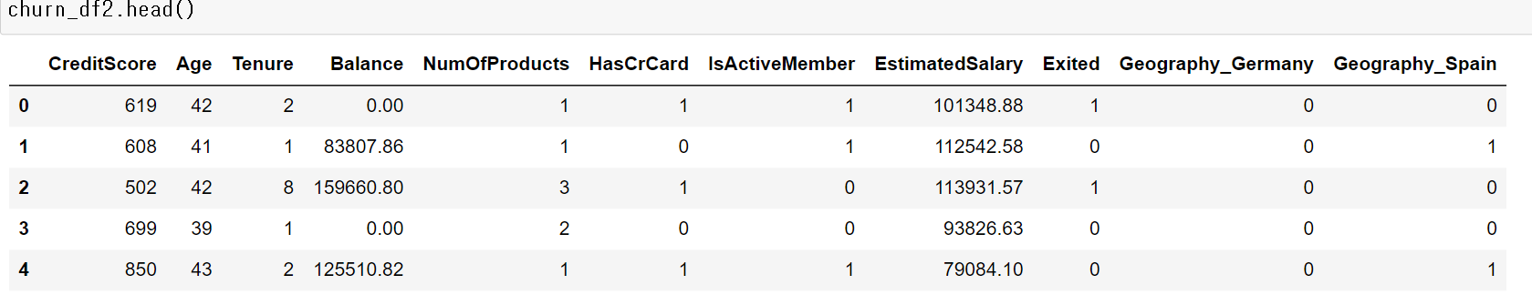
4. split data
# Define the y (target) variable
y = churn_df2["Exited"]

# Define the X (predictor) variables
X = churn_df2.copy()
X = X.drop("Exited", axis = 1)

# Split into train and test sets
X_train, X_test, y_train, y_test = train_test_split(X, y, test_size=0.25,
                                                    stratify=y, random_state=42)
5. modeling
-cross-validated hyperparameter tuning
xgb = XGBClassifier(objective='binary:logistic', random_state=0)

cv_params = {'max_depth': [4,5,6,7,8],
             'min_child_weight': [1,2,3,4,5],
             'learning_rate': [0.1, 0.2, 0.3],
             'n_estimators': [75, 100, 125]
             }

scoring = {'accuracy', 'precision', 'recall', 'f1'}

xgb_cv = GridSearchCV(xgb, cv_params, scoring=scoring, cv=5, refit='f1')
-학습(시간 30분 소요)
%%time
xgb_cv.fit(X_train, y_train)
6. 피클
1) 저장 위치
path='/work'2) 파일 쓰기
with open(path + 'xgb_cv_model.pickle', 'wb') as to_write:
    pickle.dump(xgb_cv, to_write)
3) 파일 읽기
with open(path+'xgb_cv_model.pickle', 'rb') as to_read:
    xgb_cv = pickle.load(to_read)
4) 다른 모델 파일 읽기
# Open pickled random forest model
with open(path+'rf_cv_model.pickle', 'rb') as to_read:
    rf_cv = pickle.load(to_read)

rf_cv.fit(X_train, y_train)

print('F1 score random forest CV: ', rf_cv.best_score_)
print('F1 score XGB CV: ', xgb_cv.best_score_)
F1 score random forest CV: 0.580528563620339
F1 score XGB CV: 0.5838246640284066
CPU times: user 18min 50s, sys: 3.56 s, total: 18min 53s
Wall time: 18min 53s
7. 교차검증 평가
def make_results(model_name, model_object):
    # Get all the results from the CV and put them in a df
    cv_results = pd.DataFrame(model_object.cv_results_)

    # Isolate the row of the df with the max(mean f1 score)
    best_estimator_results = cv_results.iloc[cv_results['mean_test_f1'].idxmax(), :]

    # Extract accuracy, precision, recall, and f1 score from that row
    f1 = best_estimator_results.mean_test_f1
    recall = best_estimator_results.mean_test_recall
    precision = best_estimator_results.mean_test_precision
    accuracy = best_estimator_results.mean_test_accuracy

    # Create table of results
    table = pd.DataFrame()
    table = table.append({'Model': model_name,
                        'F1': f1,
                        'Recall': recall,
                        'Precision': precision,
                        'Accuracy': accuracy
                        },
                        ignore_index=True
                       )

    return table

xgb_cv_results = make_results('XGBoost CV', xgb_cv)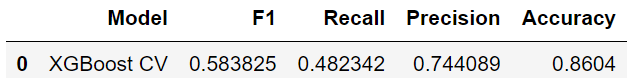
8. ytest로 평가
# Predict on test data
xgb_cv_preds = xgb_cv.predict(X_test)
print('F1 score final XGB model: ', f1_score(y_test, xgb_cv_preds))
print('Recall score final XGB model: ', recall_score(y_test, xgb_cv_preds))
print('Precision score final XGB model: ', precision_score(y_test, xgb_cv_preds))
print('Accuracy score final XGB model: ', accuracy_score(y_test, xgb_cv_preds))
9. 혼동행렬
# Create helper function to plot confusion matrix
def conf_matrix_plot(model, x_data, y_data):
    model_pred = model.predict(x_data)
    cm = confusion_matrix(y_data, model_pred, labels=model.classes_)
    disp = ConfusionMatrixDisplay(confusion_matrix=cm,
                             display_labels=model.classes_)

    disp.plot()
    plt.show()
conf_matrix_plot(xgb_cv, X_test, y_test)
10. feature importance
plot_importance(xgb_cv.best_estimator_);